
Last month, we took a close look at Skew-T (sounding) diagrams and how they’re constructed. To refresh your memory, Skew-T’s are simply diagrams showing a vertical profile of temperature and moisture at a given station at a given time. The up direction is increasing altitude, and the right-hand direction is increasing temperature or moisture. The data for the diagram is most often obtained using balloonlaunched radiosondes, but simulated Skew-Ts can be produced using analysis and numerical models.
These diagrams might seem intimidating, but they’re very easily found on the Internet, and sites like Pivotal‑Weather.com let you click on the numerical forecast maps along your route of flight and see a Skew-T. They can easily be brought up on any phone or tablet, and they’re provided as a single image that literally gives a myriad of keys and clues to the forecast puzzle unlike any other weather chart. How could you not pass this up?
Deadly Ice Flight
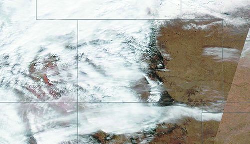
Halloween 1994 was a dreary day across much of the Midwest. A low pressure system was located in southern Illinois, with a warm front extending east into southern Indiana and Ohio. Conditions were mostly IFR and MVFR, and temperatures struggled to reach the 50s and 60s. It looked like grim prospects for trick-or-treating.
Our case begins in Indianapolis, where an American Eagle ATR-72’s young crew had flown in shortly before 1 p.m. The crew had a brief lunch, with a scheduled departure time of 2:10 p.m. for Chicago. Conditions at Indianapolis were 1300 feet overcast and five-miles visibility in fog, with a temperature near 60. The weather was much the same in Chicago, with temperatures in the 40s.
The flight was delayed by 45 minutes but was soon up in the air and was cleared to 14,000 feet and soon afterward to 16,000 feet. The plane never left the dense nimbostratus overcast. After topping at that altitude for five minutes, the plane was cleared down to 10,000 feet. The ATR-72’s icing system was switched on. The plane leveled off at 10,000 feet at 3:18 pm, and was routed into a series of holding patterns in the clouds. About ten minutes into these holds, the CVR detected the sound of music in the first officer’s headset and a flight attendant chatting with the pilot. This hold was clearly overshadowed by monotony.
The first sign of trouble came at 3:33 p.m. when the pilot commented about the high deck angle in the turns. “We’re just wallowing in the air right now,” he observed. For the next ten minutes, the crew continued through the holds. The first officer made occasional mention of some ice that was observed, and the deicing system was activated again.
At 3:56 pm ATC instructed the crew to descend and maintain 8000 feet. About a minute later, the flap overspeed warning sounded. Expecting this, the pilot set the flaps to the zero- degree position. The loss of lift, combined with heavy ice on the wings caused the airplane to seek a higher angle of attack. This led to a stall and a series of sharp rolls, followed by a downward plunge. Falling out of the sky like a rock, the aircraft impacted a 20-acre soybean field 38 degrees nose-down and partially inverted at a speed of 375 knots. All 64 passengers and four crew members perished in the crash.
Deadly Ice Skew-T
Let’s look at the Skew-T (previous page) for the morning of the incident. This sounding is for Peoria, Illinois, located about 120 miles to the west. As weather tends to move west-to-east, this sounding would provide an acceptably accurate approximation of conditions over Indiana eight hours later.
To make this analysis easy, we’ve enhanced it with a height scale on the right and three colors of shading. The yellow color corresponds to temperatures above freezing, the darker blue band for temperatures between -20 and zero degrees C, the critical icing zone, favorable for clear ice. The lighter blue (cyan) band shows temperatures below -20°C, usually associated with rime icing and low water content.
Looking at the temperature line on the right, we see immediately at a glance that temperatures are cold near the surface, but not quite freezing. The line bends sharply to the right as we ascend from 3000 feet to 5000 feet, indicating a frontal inversion. This means that the entire sounding below 5000 feet is located within a frontal zone.
What kind of front? Just look at the wind scale to the right. The easterly wind within the frontal zone tells us that a warm front is close by, lurking maybe 100 to 200 miles to the south. If it was a cold front we would see westerly or northerly winds in this band instead. Pretty easy, right?
At 5000 feet (850 mb) the temperature climbs to its highest value, almost five degrees C. This marks the top of the frontal zone. From here upward, we’re in tropical air, though of course at this altitude in October it’s not going to feel quite like the beach in Cancun.
We can see that at roughly 9000 feet, the temperature line crosses over below freezing. If there’s enough moisture and lift, we can have serious icing problems here. The temperature continues to fall, crossing out of the band into -20 temperatures at about 21,000 feet. We find another sharp inversion at about 32,000 ft. This is the tropopause. Above this layer is the stratosphere.
Above the frontal zone (above 5000 feet) we see that the winds are southwesterly. A southwest or south wind here indicates upper-level troughing is to our west and that the trend is likely to be deterioration of the weather, though that could take hours or days. Also of note is the 100-knot winds around 40,000 feet, indicating we have a polar jet in the area. It’s almost certainly linked to that low-pressure system in Illinois we talked about in the story.
Now look at the moisture line on the left. Notice how closely it follows the temperature line. This is a sign of very high relative humidity. In fact, if the lines are within about five-degrees Celsius of each other, this is always an indication of clouds. In this example, the lines are within two to four degrees of each other up to 20,000 feet, which corresponds to a relative humidity of about 90 percent, close enough to saturation. There’s probably cloud material here, and all it takes is a little lift for the cloud droplets to coalesce and collide to produce supercooled and liquid drops.
Now follow along with the story on the Skew-T and you’ll get a picture of what happened. The airplane remained mostly in the critical icing band, then held for 40 minutes in a zone where the temperature was about -2 and abundant moisture was present.
Granted, the sounding doesn’t tell us anything about the kind of lift working on the air mass, which is one of the key factors that produces large supercooled
drops that give us severe icing. That’s not a problem though because the Skew-T is just one of many tools that you can use. It won’t forecast icing by itself, but it will give you clear information on how the atmosphere is structured and which layers have the potential for icing.
Extreme CAT Flight
As we all know, many days in aviation come alive while the city sleeps. Such was the case on December 9, 1992 when our three-man crew sorted out their flight plan at Emery Worldwide air freight center, located on the north side of Dayton International Airport. The DC-8 Series 50 cargo jet N810CK, operated by Kalitta Air (callsign Connie), was loaded with 20 tons of cargo. It was already looking like a long day ahead, as the morning had started hours earlier with a short leg from Toledo.
With the December morning cold, gray, and dreary, Connie 926 took off around 7:30 a.m., climbed out of the overcast, and pointed west for the fivehour flight, reaching FL280. As they neared Kansas City above an extensive overcast, the flight gradually started picking up clear air turbulence (CAT). This slowly ramped up to a constant, annoying moderate chop that continued incessantly over the next 45 minutes.
Nearing the Goodland VOR in northwest Kansas, the crew requested FL310 and were approved. Unfortunately as the flight continued there wasn’t much change in the turbulence. Ironically, a TWA flight nearby wasn’t happy with their bumpy ride either, and requested a descent to FL290. Passing over the Denver sector, the crew felt apprehension at the radio traffic they were hearing. A Boeing 727 climbing out of Denver reported fighting through severe turbulence on their climb up to cruise level, while a UPS flight said they were “getting beat up pretty good.” The turbulence was worsening and the DC-8 was getting firmly bounced around.
Passing high over the western suburbs of Denver just after 8 a.m. Mountain
Time, Connie 926 suddenly pitched up, then slammed backed down, redlining the airspeed, and the aircraft was knocked into a series of violent 20-degree rolls that pushed the crew against their harnesses. The pilot radioed to the sector controller, “We need lower right now!” Suddenly the Number 1 engine fire bell rang out. The crew retarded the engine and followed the shutdown list, then asked for an emergency landing at Denver.
The chaos and the continued turbulence left no time to dump the remaining three hours of fuel. The airplane would have to be landed heavy. The crew made a swift descent into the Stapleton terminal area and rolled onto final approach. Spotting the aircraft just a few miles away, Stapleton Tower came on the radio: “Connie 926 heavy, Runway 26L cleared to land, and just so you know, the number one engine is missing from the aircraft.”
Fortunately there is a happy ending: Connie 926 completed a safe landing, and was met by the airport fire department. The 2-ton Pratt & Whitney JT3D engine was never found. Our best guess is the pile of metal was eventually discovered by puzzled hikers in the rugged valleys around Bergen Park.
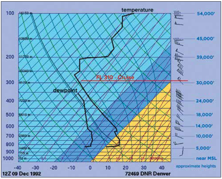
Extreme CAT Skew-T
The Skew-T for Denver (above) was provided by a balloon launch just a couple of hours earlier. This provides an almost perfect sample of the air mass that Connie 926 flew through.
We can start out by first looking at the temperature line, the thick vertical line on the right side. Working from the bottom, we can see that the line takes a sharp rightward slope, indicating warmer air just a few hundred feet above the surface. This is the radiational inversion, which marks a separation between air near the surface cooled by nighttime radiation, and the prevailing air mass above. If the ground was wet with recent rainfall, we would likely have seen shallow morning fog.
Above the radiational inversion we see the air mass start to cool with height. At about 14,000 feet we reach a layer where the temperature line slopes far to the left. This shows very strong cooling with height and the potential for strong instability. In fact it almost matches the slope of the dry adiabats, the thin guidelines that slope from lower right to upper left. This is significant because the dry adiabats represent the maximum possible rate of cooling that the air mass can support.
Using the Skew-T we can see this very unstable layer spans 14,000 feet to 34,000 feet MSL. It looks like things stabilize rapidly at the tropopause at 38,000 feet, and above that there is a good chance of getting into much smoother air. If you had flown this day, you stood a good chance of escaping most of the turbulence if you could reach 41,000 feet. That inversion above the tropopause would help dampen out a lot of the rough vertical motion.
We can see that icing is likely not a problem. The dewpoint and temperature lines are not packed close together as with the ATR-72 case study above. In this case the lines are about 15 degrees Celsius apart, suggesting relative humidities of below 50 percent. It’s very unlikely that there are any clouds in the critical icing layer, so icing would not be forecast.
However what’s most important is the wind plot on the right side. Notice how wind speeds average about 40 knots from 20,000 feet to 30,000 feet, then increase substantially to 90 knots at 33,000 feet. This tremendous increase over such a short vertical distance is the smoking gun that explains why Connie 926’s engine was torn off its wings. Almost every CAT forecasting guideline emphasizes vertical shear, and here you can see it on the Skew-T, directly observed by the radiosonde instrument.
Although the Skew-T does not suggest much vertical shear at lower altitudes, the combination of strong static instability plus the moderate flow directly perpendicular to the Rockies was what provided a classic mountain wave setup. These mountain waves easily propagated downstream to higher altitudes in the unstable air. The zone of
strong shear at cruise altitude was the icing on the cake.
In Closing
Interestingly, the saga of Connie 926 with local news headlines captured the attention of the National Center for Atmospheric Research, in nearby Boulder, and helped spark a renaissance in turbulence forecasting. Before 1992, turbulence forecasting mostly relied on rules of thumb. Today, thanks to the advances in microphysics and numerical forecasting, we have sophisticated graphical turbulence guidance products available on
sites like AviationWeather.gov.
Have we made a believer of you? The Skew-T is a highly capable tool, and in my own forecast use I refer to them every day as they provide all kinds of unique insight about what’s going on. They literally are the playbook at a given station for the day. Over the two years in IFR Magazine we’ve provided at least three other articles on how to use this diagram, one of them from another experienced author, so you’ll definitely want to get your hands on some back issues and learn what these tools have to offer.


Excellent concise review of the Skew-T interpretation. Thanks!