
These WX SMARTS articles typically focus on big weather makers like fronts, systems, thunderstorms, and the weather they all produce. But atmospheric stability is a less-talked-about process that works in the background and “primes” the atmosphere in many ways. While you might dodge thunderstorms and fly past frontal zones, stability (and the lack of it) is embedded in all parts of the atmosphere. You can’t escape it even in clear weather.
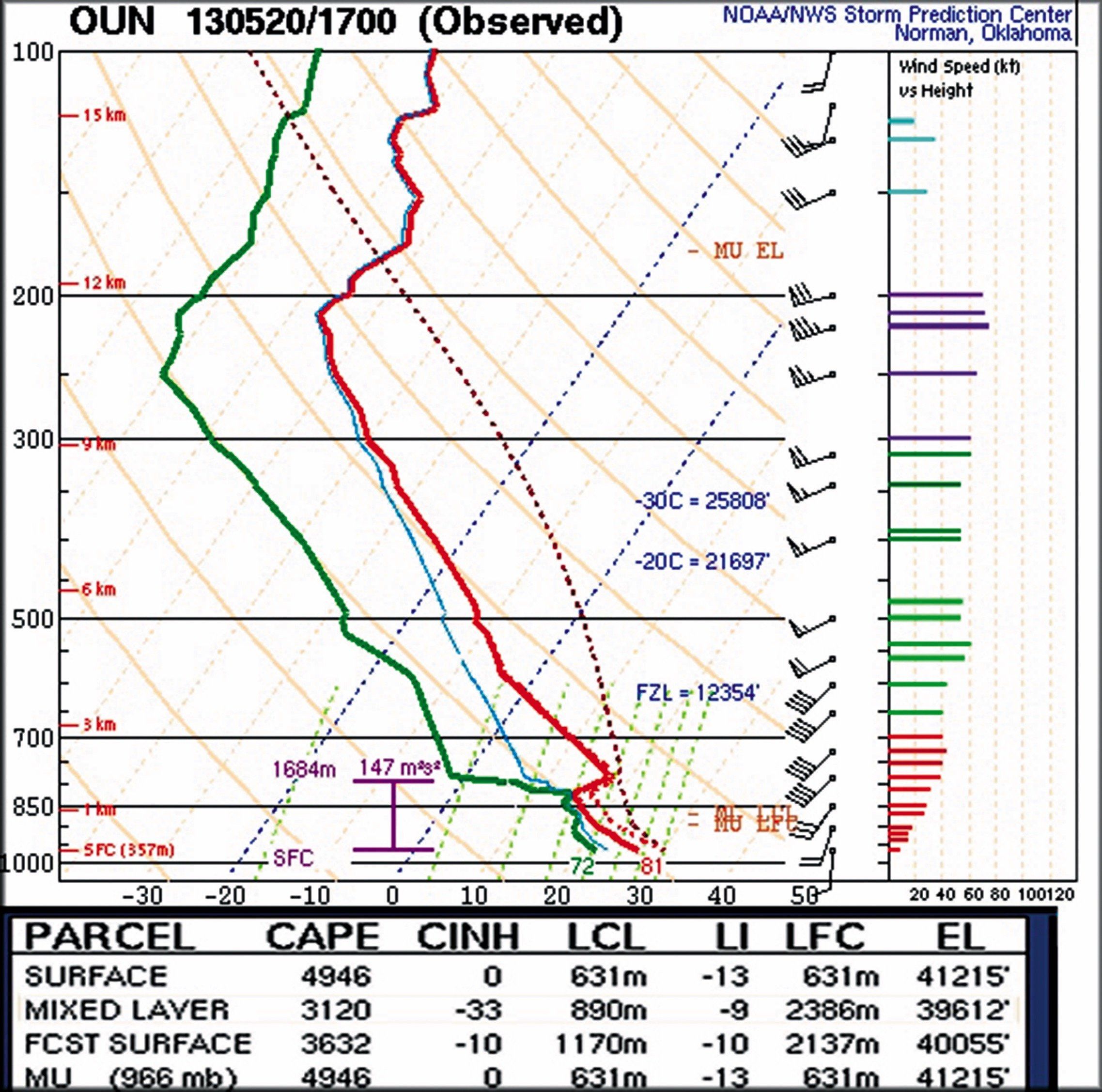
While stability and instability don’t always cause weather, they leave a mark on even VFR forecasts in many subtle ways, and they influence everything from wind gusts to cloud layers. Even in forecast models, there are always complex equations that factor in stability. Stability is important enough that an entire chapter is dedicated to it in the FAA’s Aviation Meteorology circular. For meteorologists, a chart known as the Skew-T diagram is used every day at forecast centers. It’s literally a worksheet that helps forecasters visualize the day’s stability and make calculations on it.
I’ve increasingly noticed that both pilots and aspiring meteorologists most often struggle with stability and Skew-T’s. Maybe it’s because this is where we enter the mysterious world of thermodynamics. It’s a shame people shy away from the subject, as stability offers extensive information once you have a solid understanding of the underlying principles and know how to use the available tools. Fortunately I’ve found stability can be taught quickly using the basics and taking a practical approach.
Now that it’s spring and weather is ramping up, this is a perfect time to dig into it. Thunderstorms, crosswinds, gusty winds, fog, and low ceilings are all tied to stability in the atmosphere and its distribution at different levels.
Meet the Parcel
We’ll start with the most basic element, the parcel. Working with stability, we often use an imaginary, arbitrary volume of air meteorologists widely call a “parcel.” For everyday purposes we can picture a parcel of air as being the size of a large box or a balloon. The stability numbers like CAPE and Lifted Index, seen on some forecasting sites measure the changes that a parcel undergoes during its trip through the atmosphere.
It’s important to understand that the parcel and the environment are two separate systems. A lot of the confusion I see comes from this not being made clear in training materials. The environment is just a snapshot of the atmosphere in your area of interest. When we receive radiosonde data showing temperatures and winds, look at a winds aloft chart, or even when we see a METAR, we are looking at conditions in the environment.
Parcels begin as part of the environment, but in analyzing stability we select parcels and conceptually “detach” them, like cutting an article out of a newspaper. Maybe the parcel is moved; maybe moisture is added. But whatever the case, the parcel begins as a sample of the environment that undergoes some motion or change. The parcel might ultimately represent a cloud, wind gusts, updrafts and downdrafts, localized weather conditions, or even a storm.
Static Stability
The basic concept of static stability describes the character of a layer of environmental air of some arbitrary depth. The lapse rate is used to measure static stability, or the change in temperature per unit of vertical distance. In a standard atmosphere the temperature decreases by about 3.6 degrees F per 1000 feet. This is a natural occurrence because pressure in the atmosphere decreases with height, and the temperature must decrease as a result.
If the temperature decrease with height is unusually strong, this is a high lapse rate, sometimes called a “steep lapse rate” by meteorologists. This always indicates high static instability, effectively giving us an unstable environment. Likewise if the temperature decreases slowly or even increases with height, this is high static stability. The environment is considered stable.
Why is this so? This is where our friend the air parcel comes in.
Let’s take an environment with high static instability. We’ll assume the layer extends from 0 to 5000 feet and cools from 90 degrees F at the bottom to 40 degrees at the top, giving us a lapse rate of 10 degrees per 1000 feet. Let’s imagine detaching a parcel from the bottom of this layer and forcing it to rise to the top. Will it cool to 40 degrees when it gets to 5000 feet? No. Here’s why.
A parcel is always treated as a closed system, with no heat or moisture added. When it rises to 5000 feet it has no way of “knowing” the existing temperature at that level, nor can it cool itself down to the ambient temperature. It also doesn’t cool for the same reasons as the environment. The existing air at 5000 feet might have originated at jet stream levels over a mountainous area then descended to 5000 feet. Meanwhile our parcel might have originated down below from a desert plain. So the two volumes of air have different histories, and there’s no specific reason for the parcel to cool.
Adiabatic Cooling
But the air does cool, because changes in pressure and volume do act on the parcel, as shown by the ideal gas law. Adiabatic cooling and warming take place whenever the altitude of the parcel (thereby its pressure) changes. This occurs at a fixed, predictable rate. We call this the adiabatic lapse rate. In a dry atmosphere this is about 5.4 degrees F per 1000 feet. (These numbers aren’t constants, by the way. They vary a little bit at different levels and temperatures). The temperature change tells us exactly what the final temperature of our parcel will be. It cools by (5.4 1000 5000) 27 degrees F, so the final temperature of the parcel will be (90 − 27) 63 degrees.
Now look at the situation we’ve created. At 5000 feet, the environment is 40 degrees, while the parcel is 63 degrees. This is where buoyancy comes in. If you picture this parcel as a 63-degree balloon, you can see that it has a lot of buoyancy (heat rises). Buoyancy means acceleration of the air, giving us motion that we call convection.
It’s easy to see that the example we’ve given could represent a cumulus cloud, and that the cloud will probably grow rapidly into a thunderstorm if there’s enough moisture. Now you understand how static instability translates to turbulence, weather, and upward motion. In fact, clear air turbulence has a strong association with static instability in layers aloft.
This also works in the other direction. Let’s carve out a parcel in the environment at 5000 feet, where it’s 40 degrees. If we push the parcel down to sea level, it warms adiabatically by 27 degrees, giving it a final temperature of 67 degrees. If you compare this to the 90F environment, the parcel clearly has a lot of downward buoyancy. This is a great representation of a thunderstorm downdraft or microburst. So high static instability is always favorable for vertical motion, whether it’s upward or downward. We often refer to an atmosphere with high static instability as an “unstable atmosphere.”
The Stable Version
Let’s now create a layer with high static stability. A stable atmosphere might have a temperature of 60 degrees at the ground, with 65 degrees at 5000 feet. Notice the temperature is increasing with height. We refer to this as an inversion, since the usual temperature progression is cooler aloft.
So what happens when we lift a parcel from the ground? It starts out at 60 degrees, cools by 27 degrees, and finishes at 33 degrees at 5000 feet. If we compare that to the 65-degree environment, we can see the parcel is much colder than the air around it. If it were a balloon, instead of rising faster it would sink. Reaching sea level again it would return to its 60-degree temperature, same as the environment, and it is no longer accelerating downward.
Statically stable layers resist vertical motion. Parcels will cling to their original level. If they get displaced, perhaps moving over a mountain, the parcels will move back to their original level, oscillating back and forth until they regain equilibrium. This oscillating effect often produces spectacular waves in the cloud layers.
The resistance to vertical motion is why visibility is often impaired during stable weather. Fog, haze, and pollutants get stuck near the ground because air currents can’t move upward and disperse particles into the free atmosphere. This is a common occurrence across North America during the cool season, especially in the arctic regions where inversions can be severe, and in the western states where mountains restrict even the horizontal dispersion of fog and haze.
Stability Affects Weather
The effects on weather by stability are profound. Let’s take the example of stable air near the ground. As we’ve shown, it suppresses vertical motion and favors deteriorating visibility due to fog, haze, and smoke. This also prevents wind forces from interacting at different levels and suppresses convection, so wind gusts and turbulence are unlikely. You’ll get a smooth ride.
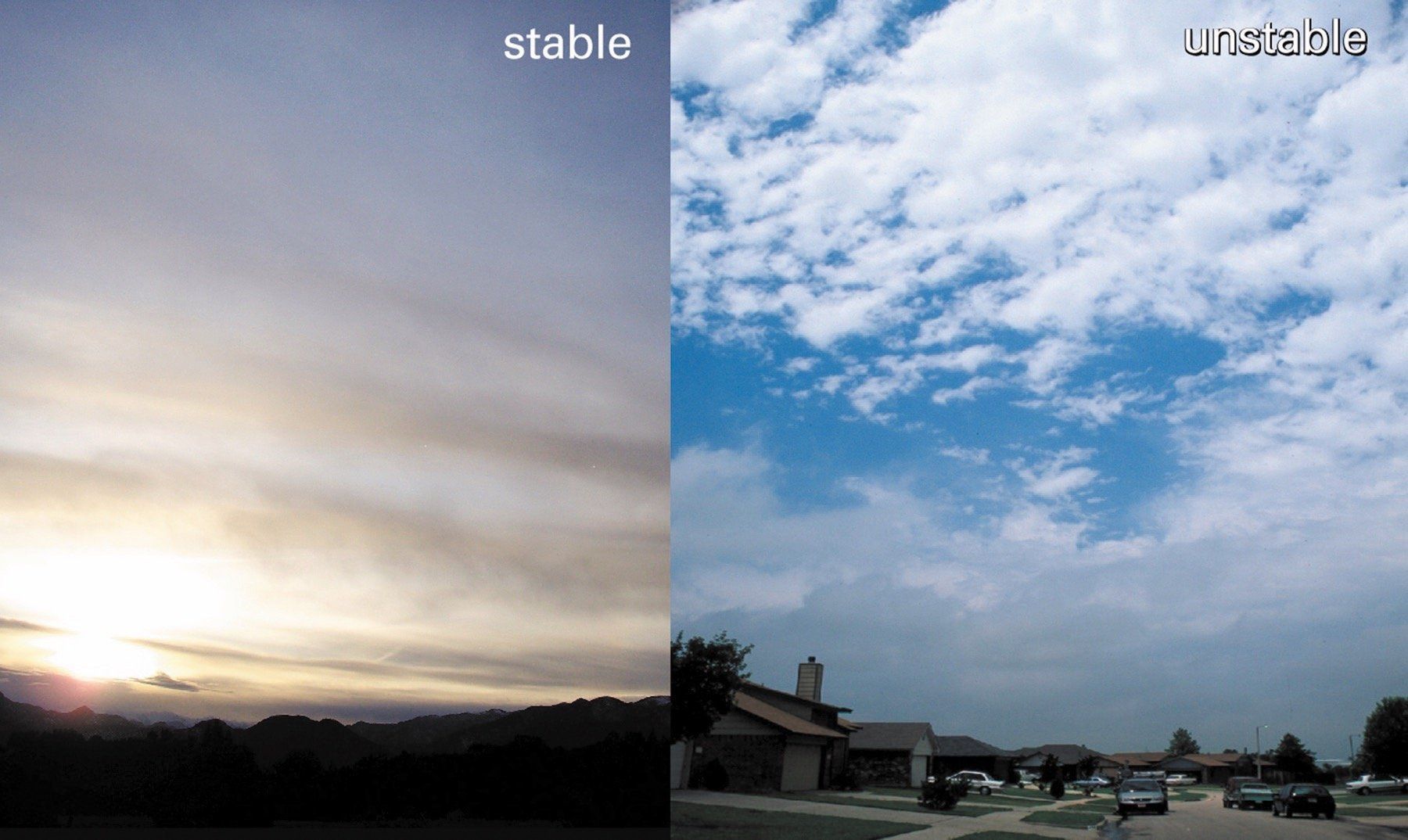
We can’t determine anything about cloud coverage, but since convection is suppressed, cumuliform clouds are unlikely. Convection might not be present but vertical motion can still occur from orography and complex mechanisms such as isentropic lift. When this happens you’ll see a lot of stratiform layers such as stratus, nimbostratus, and altostratus.
Next, let’s look at an unstable layer. Vertical motion is extensive, and we might visualize it as being prone to churning. If the layer is deep enough, fog, haze, and smoke will disperse. This means very good visibility. If you’ve ever been in the zone of instability right behind a strong cold front in the Midwest, you might have contemplated the mystery of why large cumulus clouds are growing and forming snow showers, yet somehow the sky is clear with visibility up to 50 miles or more.
Due to the deep motion, unstable layers naturally favor wind gusts and turbulence. This is especially true if there is solar heating. A gust being reported in the METAR observation indicates there are at least nine knots between peaks and lulls, and is a great indicator of an unstable layer anchored at the ground.
Since unstable layers are associated with buoyancy and convection, there are likely to be cumulus, cumulonimbus, and stratocumulus clouds. In drier climates the relative humidity is often too low for moisture to condense, so skies might be clear but there will be the same churning motion occurring invisibly in the atmosphere.
Stability Indices
Many of you may have heard of the stability index. There are dozens, if not hundreds of them, and they’re often used as rough guides for storm prediction. One of the most basic ones you might see on websites is the Vertical Totals Index, or VT. This is simply a measure of the environmental lapse rate between roughly 5000 and 10,000 ft. It doesn’t factor in parcels, making it a very simple index for judging how responsive the low levels of the atmosphere are to vertical motion.
The more complex ones we use are Showalter Index (SI), Lifted Index (LI), and CAPE. These all lift parcels of air from near the surface and measure their temperatures against the environment. The Showalter Index and Lifted Index are falling out of use. Meteorologists now overwhelmingly use CAPE, Convective Available Potential Energy, which looks at the entire depth of the environment and expresses the result as energy in joules per kilogram. A CAPE value above 1000 usually means storms.
To see stability indices in your area, visit a website with sounding plots, likeweather.rap.ucar.edu. orweather.uwyo.edu.
Add Moisture
You might notice we’ve kept things simple by not introducing moisture. That’s where things get tricky, because if a parcel is saturated and is rising, the lapse rate falls to 2.7 degrees F per 1000 feet. Fortunately it’s not necessary to learn about this to understand stability basics, and it adds more complexity than you really need as a pilot. But it’s worthwhile to point out a few highlights.
First: the adiabatic lapse rate change of roughly 5.3 to 2.7 occurs because 2.6 degrees of extra heat is being added to the parcel. You may have heard of the term “latent heat,” and that’s exactly what this is. It’s the molecular heat given off by the phase change when water vapor condenses into cloud droplets. It’s an extremely important process in thunderstorms and hurricanes. By adding this latent heat, parcels get a push of extra effective buoyancy, ramping up the effects of instability. It can add energy while descending, too, if rain drops are able to evaporate. Layers of dry air are good for this—this is how we get haboob storms in Phoenix.
It also means that dewpoint—that often-neglected part of the METAR—is very important during the warm season and during severe-weather episodes. The closer the dewpoint and temperature are together, the lower the dewpoint depression and the higher the relative humidity and the less vertical distance a parcel has to rise before it begins releasing latent heat. Granted, the dewpoint depression is normally low and relative humidity is high in the mornings, but the nighttime radiational inversion keeps a lid on things. You have to wait until it burns off in the morning and the low-levels begin mixing to see how temperature and dewpoint are shaping up.
All this might not sound like much, but it’s considered the bedrock of weather forecasting and it affects what kind of flying day you have. It’s also a springboard for going even deeper into moisture, air mass modification, and the Skew-T chart. We’ll cover all this in upcoming articles and show how these ingredients affect the forecast.
Tim Vasquez trained dozens of incoming aviation forecasters during his Air Force career, and got them through the mysteries of instability. He now lives in Palestine, Texas, and still has Skew-T charts on his desk.


