
Once again we delve into aviation accidents. The official 2019 numbers won’t be out until November, but the 2018 NTSB release showed there were 1347 accidents with 393 fatalities. The vast majority of these, as we might expect, were general-aviation accidents, with a sizable number of them due to weather. The airlines, charter operators, and medical services didn’t escape unscathed, having logged 72 accidents.
With aircraft continuing to have accidents, there’s still plenty of work to do to emphasize safety. Our focus in Wx Smarts is on the weather picture. And one of the best ways to drive the point home and teach the hazards is using real-life stories about pilots perhaps not unlike you. Our analyses here aren’t specifically about the accidents, but instead about the weather as it played a factor and how the pilot might have safely navigated the existing conditions.
A Florida Windstorm
Our case study for this issue takes place on a turbulent, unsettled Thursday afternoon in November in Ocala, Florida, located about 50 miles northwest of Orlando. The pilot was a 73-year old retiree who owned a 1968 Mooney M20 Ranger.
His plan was to fly to Jacksonville, Florida, about 80 miles northeast, to visit for his daughter’s birthday and enjoy a family Thanksgiving gathering. The pilot had logged 3150 flight hours with 520 hours of instrument time. About 400 flight hours were in the Mooney.
Ocala was just a stopover to drop off his passenger. Although the flight was uneventful, the sky was threatening during the landing. Almost immediately after landing, the winds began gusting and the rain began pouring.
The pilot planned to continue solo for the final leg to Jacksonville. He waited in the FBO for things to clear. The rain was slow to ease up.
While waiting for the rain to stop, the pilot asked the FBO for fuel. The attendant explained that it would be better to wait out the weather. The pilot insisted, saying he needed the fuel soon as he was trying to get to his daughter’s house.
He proposed they fill up in the rain underneath an umbrella, while lining the fuel cap with a towel. The attendant put in a call to the technicians and they agreed. The fueling job was completed around 1:30 p.m.
About 30 minutes later, the pilot filed a flight plan. He did not get a weather briefing. Investigators were unable to find any weather sources that he might have reviewed.
With the rain tapering off, the pilot fired up his airplane to continue the journey. At 2:19 p.m. the aircraft was off the ground and the pilot contacted Jacksonville Approach. He was radar-identified and instructed to proceed direct to Cecil Field at 3000 feet, and expect an ILS approach to Runway 36R.
Over the next 10 minutes, the airplane flew an erratic, wandering path with large deviations to the left of the track. The controller grew concerned and discussed it with the pilot. “Your target’s going all over the place. Are you having issues?”
“Yeah. This wind is giving me hell. I’m getting on it.”
“Roger, just let me know if you need assistance.”
“I’m good, thank you.”
At 2:59 the airplane was handed off to Cecil Tower. At 3:03 the pilot broke off the approach and asked to try again. “Roger, ah, amend the altitude. Maintain 2000 and expect vectors for the ILS Runway 36R approach. Fly heading 220.”
The airplane made a lumbering left turn southwest. About a minute later, the controller grew concerned about the plane’s low altitude. “Say altitude.”
“I’m busy right now, let me get leveled out.” Then came, “Fifteen hundred.”
At 3:13 the controller offered Jacksonville International Airport, where the ceiling and visibility were better. The pilot accepted. “Okay, that’ll work. Let’s go to Jax.”
“Roger, and when able fly heading 040 for vectors for the ILS Runway 8 approach.”
“040,” he confirmed. That was the last transmission received from the airplane in spite of efforts from ATC and nearby aircraft to raise the Mooney. Within minutes ATC notified Clay County Sheriff’s Office. Military police at Camp Blanding were notified, and they located the wreckage about two hours later in a wide field. Toxicology reports showed no substances in the pilot’s system, and the aircraft was determined to have no defects that might have caused it to crash.
A Stormy Pattern
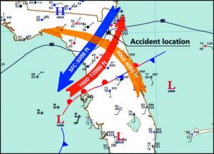
The surface chart showed a strong stationary front extending southwest to northeast across central Florida. With southerly winds near Tampa, a surface cyclone was indicated just off the west coast of Florida. Although the isobars didn’t reveal a strong circulation at the surface, upper level charts showed that the system intensified with height, shown by the arrows.
Just off the surface was a strong pressure fall in the Gulf of Mexico, which helped back the 4000-to-6000-foot winds so that they were out of the southeast. This created a band of moist “overrunning” tropical air over the warm front. Finally this was topped off above 7000 feet by strong southwesterly winds associated with a mid-level trough in Georgia. All of this created very strong directional changes through a relatively shallow layer: a potent situation for low level turbulence.
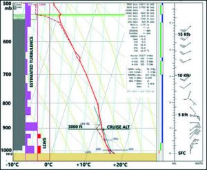
A Skew-T diagram close to the time of the accident showed temperatures of 13-degrees C at cruise altitude, with no chance of ice. However this same diagram also showed winds of 30 knots out of the northeast, giving the pilot a strong—although manageable by a Mooney—headwind. The diagram also showed strong directional shear with computed turbulence maxing out the limits of the algorithm. This is probably what gave the pilot trouble.
Complicating the situation was a band of rain showers that the pilot flew into while flying southwest to reposition for the approach. Although these clouds topped out at only 10,000 feet and strong convection was not indicated, the rippled appearance suggests transverse banding, a configuration that develops in highly sheared conditions.
The striated appearance of the weaker showers bordering large areas with no radar returns suggests embedded layers of dry air were being brought in from the east, which would result in evaporational cooling and vertical acceleration as the precipitation falls through these layers. This in turn magnifies the turbulence around these showers, allowing more vigorous overturning of layers.
Doppler Radar Clues
Although we think of NEXRAD as a tool for finding storms, it’s tremendously underused to visualize the overall wind field. One important technique used by meteorologists is to select base velocity products and use the higher tilts or higher elevations, where the antenna points 10 or 20 degrees above the horizon. This brings all the different values into a tight, compact presentation and uses scatterers close to the radar that reflect high levels of power.
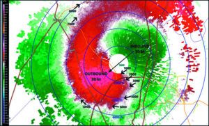
What we see in such an image gives us the environmental wind field. In our sample image we find a large, dark green (inbound) area on the northeast side of the radar, indicating winds of 30 knots originating from the northeast and blowing to the southwest, where we find a bright red (outbound) region representing the same 30 knots outbound from the radar.
To find actual values, we simply track the “zero line,” which divides the blue/green inbound shades from the reddish outbound colors. Wind flow along this zero line is always perpendicular to the radar, so simply by looking at its direction from the radar we can easily “see” the wind direction at a glance.
Remember that as we move away from the radar, we’re not interested in where we are geographically, like when we’re identifying a storm. Instead we’re more concerned with how high each radial is. This is a simple function of distance: as we move away from the radar, we find the beam at higher and higher altitudes. These have been plotted on the chart, but tools like GRLevel2 can identify heights on radar images using the mouse. Just to summarize: inner radials are close to the ground, while outer radials are high above the surface.
Using this velocity data, we get a very accurate picture of 30-knot winds from just above the surface to about 5000 feet. We also find strong turning of the wind from 3000 to 7000 feet. We don’t need to even track the twists and turns of the zero line, we can simply see that it forms a spiral shape that always indicates directional shear with height. This is especially true if strong winds are being displayed, like the bright red and dark green shading. Severe storm forecasters are familiar with the spiraling of velocity patterns in tornadic weather environments, caused by strong low-level shear.
Not surprisingly, directional shear and speed shear between the top and bottom of a layer, in the presence of strong wind velocity and instability, is known to be one of the best indicators of turbulence. In fact, an NTSB report analyzed this layer of turning winds and found that the computed shear values corresponded to severe to extreme turbulence in the 3000 to 5000-foot layer.
If you find velocity products a bit too challenging, NEXRAD offers a product that simplifies a lot of this. It’s called the VAD/VWP product (Velocity Azimuth Display Wind Profile). Most radar websites skip it, but you can find it on sites like weather.cod.edu/satrad and on commercial subscription services like WeatherTap. This displays wind plots on a time-versus-altitude grid.
You can use the VAD/VWP product to get an idea of winds for your flight and see how they compare to your briefing. This data is observed by the radar and is highly accurate, unless the winds are not the same on all quadrants of the radar. This is why I’ll often check the base velocity data to look for symmetry; if the colors and zero line look symmetric, then I know the VAD/VWP product is going to nail the wind data. And since the data is plotted minute-by-minute, you can easily spot changes in wind strength at various levels.
But there are a few drawbacks. There need to be scatterers visible to the radar, so there needs to be precipitation or wet clouds in the area, or the radar needs to be operating in clear air mode where it has more sensitivity. Another problem is since the plots are done in altitude intervals of 1000 feet, we don’t see the sort of fine-grained detail that we do on the base velocity graphic for the accident aircraft, and it’s harder to see low-level shear.
But for day-to-day flying, I recommend the VAD/VWP product. I do think had this pilot been able to take a look at such a product, he would have seen the low-level headwinds and the strong shear. We can’t know if it would have deterred him, but such a strongly visual format probably would have given some cause for concern.
A Final Assessment
The NTSB ruled the crash caused by spatial disorientation in IMC with a probable contributor of self-induced pressure to complete the flight.
While we can’t know exactly what happened in the last moment, we’ve made a pretty clear case that there was a rich environment for severe turbulence, the lack of a visual horizon, and perhaps some element of pilot fatigue. All of this compounded into disorientation or an unrecoverable attitude. You could have other theories that are well worth considering.
We can say the pilot in our scenario was determined and focused on getting to his destination. The fact that weather stopped him, without the classic dangers like icing or intense convection, underscores that even seemingly benign situations can bite us when we’re not prepared.
Tim Vasquez was an Air Force meteorologist who safely kept thousands of B-1B, C-130, and C-5 crews out of the worst weather. Maybe you’re not flying heavy metal, but with Wx Smarts you’ll benefit just the same.


I don’t know any pilot who has ever looked at VAD. Tthe article has nothing to do with the probable cause or contributing factor . It’s as if IFR has allowed someone to go off on a tangent unrelated to the accident merely so that person can display their mad skills at analyzing winds.
What a great opportunity to learn a little bit more about flying IFR safely. I appreciate the author’s use of a tragic example to help the rest of us avoid such a trap by analyzing what could have contributed to the accident. Having flown single-pilot IFR in turbulent IMC, I know how the piling-on of adverse circumstances puts a pilot just that much closer to an accident. Adding in the distraction of diverting, having to pull up a different approach and brief it, while trying to hold heading and altitude in extreme turbulence, probably was the straw the broke the camel’s back. There are good lessons here, and I appreciate the author sharing knowledge that was undoubtedly gained through years of education and experience that I don’t have.
State of the art winds analysis, if known to be available, would likely have not been considered. Especially, when more familiar weather information was just for the asking. One’s mindset to continue regardless, IMO, is a major factor in many accidents, and will sadly, continue to be.
This was a truly tragic event that could have been avoided. The FBO attendant’s remarks were so prescient. Had the pilot listened and opted to delay or cancel the flight, he might have celebrated his daughter’s birthday, if even a day later. The simple expediency of calling for a weather briefing would have been an additional safety factor. I keep one of Richard Collins’ observations every time I fly: the only hour that counts is the next hour. The number of hours in one’s log book is irrelevant in the face of complacency.