Again we follow in the footsteps of the late crash investigator Macarthur Job and focus on aviation accidents. This time, instead of taking a look at forecast ingredients, we’ll look at cases of where the pilots simply made the wrong decisions for the weather.
Of course, no one climbs into the cockpit expecting things to go wrong, and I would venture to say every pilot takes off confident they can handle the weather. However, NTSB files of weather-related accidents are filled with stories of overconfidence and incomplete understandings of the real situation that’s taking place. Our analyses will hopefully let you improve the record by adding your knowledge distilled from the forecasts.
A Rough Day in Missouri
Our first case takes us to a hot air balloon operator in southwest Missouri. It was a warm day in May, with scattered to broken low clouds and light west winds. The pilot of an Aerostar S-57 balloon prepared it for a flight to a neighboring town.
The forecast winds were expected to be 220 to 250 degrees at seven knots, with VFR conditions reported at nearby Springfield as SCT110. The pilot set out on a flight at 6:40 p.m., drifting east for about 30 minutes and landing his balloon in a rural subdivision around 7:20 p.m. where he provided tethered rides for residents up to a low altitude. Winds remained light during this time.
However while landing during the final ride, about 30 feet above the ground, a sudden wind rose up seemingly out of nowhere. In the pilot’s words, “a strong north wind suddenly hit the balloon.” He estimated the speeds to be about 25 mph. The balloon was carried rapidly southward, and it made a hard landing in the next field. The pilot pulled the vent line to deflate the balloon, but the wind picked up the balloon again and he was bounced out of the basket and dragged through the field. The two passengers managed to escape. As the balloon hit a tree, the pilot fell about 20 feet. He suffered a fractured pelvis and compressed vertebrae.
Outflow
Although our case relates to a hot air balloon, there are some interesting lessons to be learned here. Outflow boundaries are very small-scale phenomena and are considered firmly in the mesoscale range with life spans of tens to hundreds of miles and many minutes to hours. Up until about 20 years ago, numerical models had no ability to handle mesoscale details, and most forecasters were not trained in working with these types of weather phenomena. These hazards were handled as their own individual entities, without connecting them to the larger picture, and pattern forecasting and experience were used to forecast them.
However outflow boundaries are in the lower end of the mesoscale spectrum, near the microscale range. Numerical models still do not handle these features very well. One problem is sampling; we never have enough measurements to feed the small-scale equations. Normally the previous model runs are used to feed the current model, a technique called the first-guess method. The other problem is that the processes are not handled very well: terrain interactions, cloud physics, precipitation modeling, and more.
Lacking good data further complicates the forecast problem. Forecasters with a high workload, covering too large an area might miss important details at this scale. It’s very difficult for forecasters to anticipate timing of mesoscale features more than an hour or two out without extensive and thorough analysis.
Where Outflow Comes From
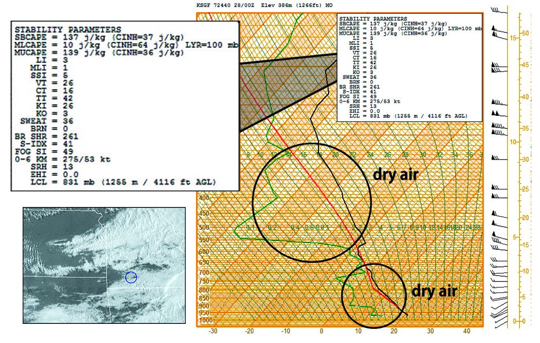
Outflow boundaries are caused by outflow air, cold pools that are generated by precipitation. The fall of precipitation through dry air can multiply the production of cold pools through evaporational cooling, so on some days with a humid atmosphere, storms will not produce noticeable cold pools, while on days with dry air aloft, cold pools can be quite large and extensive. On this particular day the upper-air sounding for Springfield showed lots of dry air, where temperature and dewpoint at various layers are widely separated. This is an excellent example of a Skew-T for a high outflow day, and it’s commonly seen in areas like Arizona and the Rockies.
It is common for outflow boundaries to move 20 to 40 miles from storms, and occasionally 100 miles or more. They die out over a half to a full day as the precipitation that’s responsible dissipates or moves elsewhere. They become almost impossible to find, though skilled forecasters can sometimes ferret them out. They can lie almost invisible and dormant for days at a time. Researchers suspect they may be part of the reason why a storm becomes tornadic while in other conditions with the same shear and instability, no tornado occurs, as they provide microscale “baroclinicity” to the storm.
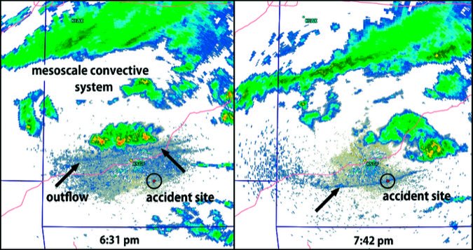
This is indeed an outflow case. The radar images 70 minutes before the accident and at the accident time show the arrival of an outflow boundary from the north. This was generated by a “mesoscale convective system,” an area of showers and weak thunderstorms in the Kansas City area earlier in the afternoon. The outflow boundary also triggered a thunderstorm in the first frame as it surged southward.
Looping the radar imagery, the outflow boundary was obvious between 5:30 and 6:00 p.m., but might have been missed by the forecasters. Radar image measurements show it was moving south at 20 mph, with no signs of decelerating as it traveled. It was still moving at 20 mph as it hit Sparta, where the balloon flights were taking place. A good rule of thumb for outflow boundaries is that maximum winds are likely to be 1.5 times as strong as the boundary movement, which suggests 30 mph gusts were likely here.
The pilot probably can’t be faulted, as it was very difficult in 2005 to self-brief and access radar information. However nowadays, radar tools like RadarScope are widely available and detailed mesoscale models like the HRRR can be viewed. It’s easier than ever to evaluate the weather before heading out, allowing one last check for last-minute hazards. Key products are close-up radar, satellite, and surface images.
A simple outflow boundary can catch pilots at the wrong place at the wrong time. Another example is the crash of a PA-46 at Chanute Field, Illinois in 2011 that we examined in August 2016.
Winter in the Rockies
Our next accident takes us a little faster and higher with a PA-32 en route from Great Falls, Montana to Scottsdale, Arizona. On board was a 56-year-old pilot who worked in the Alberta oil patch, with his wife in the passenger seat. They were headed south for a spring vacation. The pilot had 629 hours of flight time, an instrument rating and 24 hours of instrument time, but as there was no exam in the past two years he did not meet Canada’s instrument-rating requirements.
It was a blustery, mild March day in Montana and the morning temperature rose into the 50s. With cold instability and a jet stream overhead, there were extensive clouds layers all across the mountain ranges with snow showers developing along the ridgelines. Before takeoff, around 11:30 a.m., the pilot contacted Flight Service for a briefing, looking for a VFR flight at 9000 and 12,000 feet.
“I have an AIRMET for turbulence,” the forecaster said. “It has moderate turbulence below 15,000 from Great Falls until you get north of Rexburg, and then you’re out of it, so it’s only for the southwestern mountains of Montana. It looks like it’s gonna be a problem. And they still have an AIRMET for icing over the area, and that runs from Great Falls to Idaho Falls, and that says moderate icing between the freezing level and 20,000. Freezing level surface to 9000, and then I have an AIRMET for terrain obscurement … so VFR flight not recommended into areas of higher terrain obscurement.”
The aircraft took off about 15 minutes later and turned south, climbing to a cruise altitude of 9000 feet. The Big Belt Mountains, reaching almost 10,000 feet, were centered on the airplane’s path. With unstable conditions from cold air advection at 10,000 feet, clouds were crowded along the higher peaks, with bases at 7500 feet and a freezing level at 8500 feet. The tops were about 12,000 to 15,000 feet. With a 95-knot jet high above the area, the strong shear spread the humid mid-level layer into transverse bands of thick altocumulus. Visibility below was quite good as you’d expect with an unstable airmass.
Faced with clouds closing all around, the pilot took the plane slightly to the right over a 7500-foot pass, and here we saw the first altitude and airspeed deviations, with the aircraft drifting up to 10,000 feet and gradually slowing from 140 to 90 knots. The pilot then banked sharply left, turning almost 180 degrees as if to return to Great Falls. Indeed that’s what the controller thought, who notified the tower after the pilot reported he was turning back. This path took the aircraft back into the mountains.
The airplane then inexplicably began a right turn, this time approaching the higher terrain around Mount Baldy. At 10,000 feet it would have cleared the mountain range, but during the final 30 seconds, the airplane lost altitude, impacting the slopes at the 7855-foot level shortly before 12:30 p.m., about 1,000 feet below and a half mile from the ridgeline.
Flying at 120 knots into the terrain, the aircraft was torn to pieces. The pilot unfortunately was killed on impact. His wife suffered only broken ribs and had a working cell phone, and she was able to contact 911. Authorities also got a fix from the aircraft’s ELT, so rescue units were able to begin work immediately to reach the mountain slopes. However due to the severe weather conditions, it took five hours before rescue teams were able to reach her.
Analysis
Very little about the crash was unpredictable as one of hundreds of examples of controlled flight into terrain. However the computer modeling that was done nailed down a few of the hazards in much more detail than we usually get from the generalized tone of SIGMETs and AIRMETs. What is certain is all of Montana’s mountain ranges were capped with orographic clouds and mountain wave activity, and were comprised of shallow but extensive convection due to a layer of instability between the surface and 12,000 feet. The pilot took the plane into an area of dense clouds, took minimal action to keep the aircraft out of higher terrain, lost situational awareness, and the mountain did the rest.
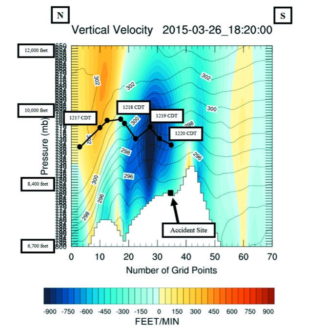
As part of the investigation, the NTSB constructed a special WRF (Weather Research & Forecasting) model for the accident. The WRF model handles terrain interaction quite well. It modeled the flow surrounding the Big Belt Mountains, and identified an area of strong upward motion, and a very large area of downward motion, where vertical velocities approached 1000 fpm. This zone combined with an aircraft heavy on fuel and weight, with a pilot trying to orient himself, were all likely factors in the outcome.
As a meteorologist, it’s not my place to say which options were best for the pilot, but this situation was clearly avoidable up until the last few minutes. Had the aircraft been capable of getting a little higher, above 12,000 feet and over the weather, or had taken a little time to wait for the weather to improve, the situation could have been much different. Unfortunately this was a flight where all the decisions went wrong. Not even the airplane’s iPad-based terrain alert software was able to help. According to the pilot’s wife, it only sounded for about two or three seconds before the crash occurred. Flying with total awareness and knowing the nuts and bolts of the weather situation before you leave the ground, rather than relying on technology, will help you make the right decisions once things start going from bad to worse.
Looking Ahead
Now that we’re getting into the heart of winter, this is a good time to get reacquainted with the basics of icing. Clear air turbulence is also rising as a threat, with a broad peak spanning December through March in the continental United States. You can look back to the February 2017 issue for turbulence or the December 2014 issue for icing. We’ll sample a little of both in the months ahead.
Meteorologist Tim Vasquez used to brief B-1B crews in the morning. Now he sleeps in and writes books and software. See his website at www.weathergraphics.com.