Skew-T Log-P diagrams(weather.rap.ucar.edu/upper). are not the most popular weather products perhaps since, at first glance, they appear confusing and hard to interpret. The diagrams are produced from atmospheric soundings, which are measurements of the vertical distribution of physical properties of the atmosphere.
As a pilot and not as a meteorologist, I find that these nomographs provide additional information about the state of the atmosphere by vertically slicing the atmosphere. Other than low-level obscuration such as fog, “nasty” weather manifests itself in the vertical. Of course, glider pilots use them extensively since an unstable atmosphere is a glider pilot’s dream. Let’s decipher these diagrams.
Soundings
First, let’s look at the following interpretation of a sounding from a February 2016 fatal weather accident in a Cessna 182 at an airport that was reporting an indefinite ceiling of 200 feet with an RVR of 2000 to 2400 feet, at or below landing minimum.
An upper air sounding from the Slidell, Louisiana, NWS site, located about 85 SM west of the accident site, depicted a moist low-level environment with saturated conditions from 500 feet AGL to 6000 feet with a capping inversion. The freezing level was identified at 14,700 feet. The wind profile indicated calm surface wind with wind from the south-southeast veering to the southwest and west through 18,000 feet. A low-level wind maximum or low-level jet was identified near 5000 feet at 215 degrees at 25 knots, with winds less than 10 knots below 1000 feet AGL.
While some of that information was not relevant (freezing level), it did indicate low-level saturation conducive to extensive fog. The NTSB report did not indicate whether the PIC involved in the accident accessed this diagram.
Source of Information
Raw data for the diagrams comes from weather balloons that are launched with effective times of 0000 and 1200 UTC. The balloons are launched about 45 minutes in advance of the effective time. Each balloon has a measuring device called a radiosonde that transmits temperature, dew point, atmospheric pressure, and wind speed to a ground station. The diagram is produced from this information, depicting both the measured data and many calculated parameters.
PRESSURE VS. ALTITUDE | |
PRESSURE | ROUNDED ALTITUDE |
200 | 39,000 |
250 | 34,000 |
300 | 30,000 |
400 | 24,000 |
500 | 18,000 |
600 | 14,000 |
700 | 10,000 |
800 | 6000 |
900 | 3000 |
925 | 2500 |
1000 | SL |
Thermodynamic Concepts
Let’s review some thermodynamic concepts. An adiabatic process occurs when neither energy nor mass is exchanged with the environment. Lapse rate is the change of temperature with a change of altitude, and the average is about 2 degrees C per 1000 feet. A positive lapse rate means that temperature decreases with altitude, whereas a negative lapse rate occurs when temperature increases with altitude as with an inversion and in the stratosphere.
Lapse rates are also determined by the amount of moisture in the atmosphere. When the atmosphere has little moisture, the dry lapse rate is about 3 degrees C per 1000 feet with lapse rates in a moist atmosphere being lower. When there is no exchange of energy with the environment, cooling of the atmosphere is due to expansion, adding another perspective: “dry adiabats” and “moist adiabats,” which are lines of constant lapse rates for unsaturated and saturated air. Confused?
Chart Dissected
Let’s first understand the axes of the Skew-T Log-P diagram. Note that the colors might vary with the source of the chart as there are no accepted standards. Reference the sample chart as we explain each element.

1. The term Skew T comes from the temperature lines (isotherms) in degrees C that are skewed from the upper right to the lower left.
2. The term Log P comes from the horizontal pressure lines (isobars) presented as a logarithmic function. These isobars are reported in millibars; see the table on the facing page for conversion to feet of altitude.
3. Wind direction (true north is “up”) and speed in knots is shown with altitude (see 2, above) using familiar flags with marks for 50, 10 and 5 knots (triangle, full line, half line, respectively). Turbulence is suggested by big differences in direction or speed at adjacent altitudes.
4. Dotted red lines represent dry adiabats where the lapse rate is around 3 degrees C per 1000 feet. Note that dry adiabats are perpendicular to the isotherms.
5. Dotted green lines represent moist adiabats. Notice that at lower altitudes the dry adiabats are approximately perpendicular to the moist adiabats, while at higher altitudes they tend to be more parallel reflecting much less moisture.
6. Dotted olive lines are saturation mixing lines; for our purposes we can ignore these lines.
7. The upper left corner is a hodograph of the movement of the balloon during its ascent in the atmosphere.
Let’s now discuss some of the sounding data most relevant to pilots that is superimposed on the diagram.
A. The solid red line shows the actual atmospheric temperature in degrees C (The tag “aa” shows the temperature at the launch site in degrees F, a mismatch of units.) When the temperature line has a positive slope, there is an inversion. Also the zero isotherm crosses the temperature line at the freezing level.
)]
B. The solid green line depicts the dew point. (Tag “bb” lists the dew point at the balloon launch site in degrees F.) Of course, the horizontal distance between the red temperature and green dew-point lines shows the spread at each altitude.
C. Lifted Index (LI) indicates the stability of the atmosphere and can be used for thunderstorm forecasting. However, it is not a perfect predictor of thunderstorms since they not only require unstable air but also moisture and a lifting mechanism. A lifted index of 6 or more is very stable atmosphere. Between 1 and 6 is still stable. When the LI is between 0 and -2, the air mass is slightly unstable and thunderstorms are possible under otherwise ideal conditions. LIs less than -2 indicate significant instability with likely thunderstorms, possibly severe if other conditions contribute.
D. K Index is an indicator of the moisture level of the atmosphere. Like the lifted index, it indicates the probability of thunderstorm formation. They should be used together and when they both suggest thunderstorms are likely, pay attention. With K-Index values (degrees C) below 20, there’s virtually no likelihood of a thunderstorm. Values between 20 and 25 suggest isolated thunderstorms are possible, with values from 26 to 30 increasing the probability to widely scattered thunderstorms. From 31 to 35 the probability increases to scattered thunderstorms and above 35 numerous storms are likely.
E. The Lifting Condensation Level (LCL) is the height at which a parcel of air becomes saturated when lifted dry adiabatically. Cloud formation is due to mechanical lifting, for example due to rising terrain, cold fronts, low pressure systems and dry lines.
F. The Convective Condensation Level (CCL) is the height where a parcel of air becomes saturated when heated from below. Both LCL and CCL provide useful information on cloud bases. The LCL is a good approximation of cloud bases for non-convective clouds that are forced to rise, whereas the CCL is a better estimate for convective clouds such as cumulus clouds. CCL is above or the same as LCL.
G. At the Level of Free Convention (LFC), a parcel of air will continue to rise without an external lifting mechanism—the parcel of air is positively buoyant. LFC levels are not always present.
H. The Equilibrium Level (EL) is the point, usually in the upper troposphere, where a parcel of air is neutrally buoyant. This usually is indicated by the tops or anvils of thunderstorms; however, thunderstorms can exceed this level by sheer momentum of the updrafts. For an EL to exist, a LFC must exist.
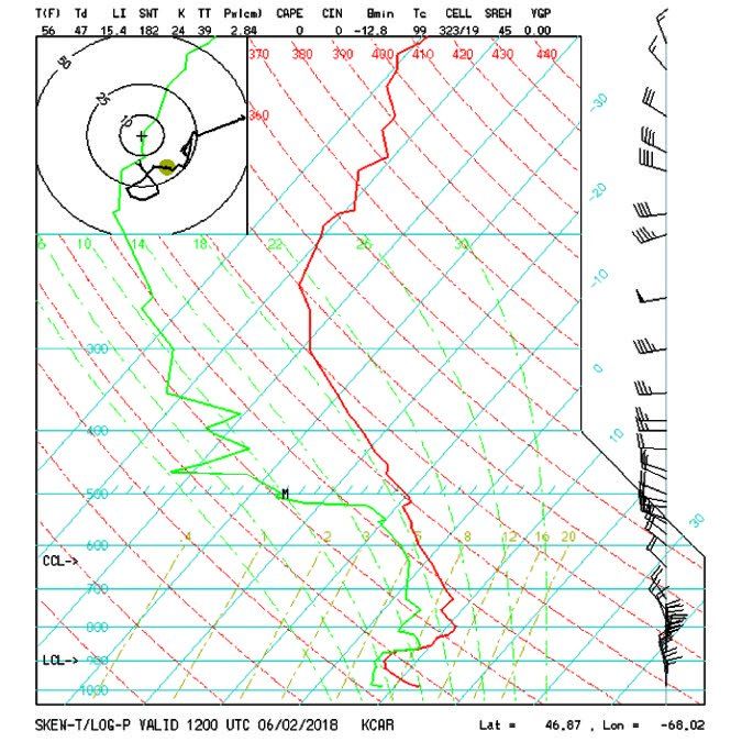
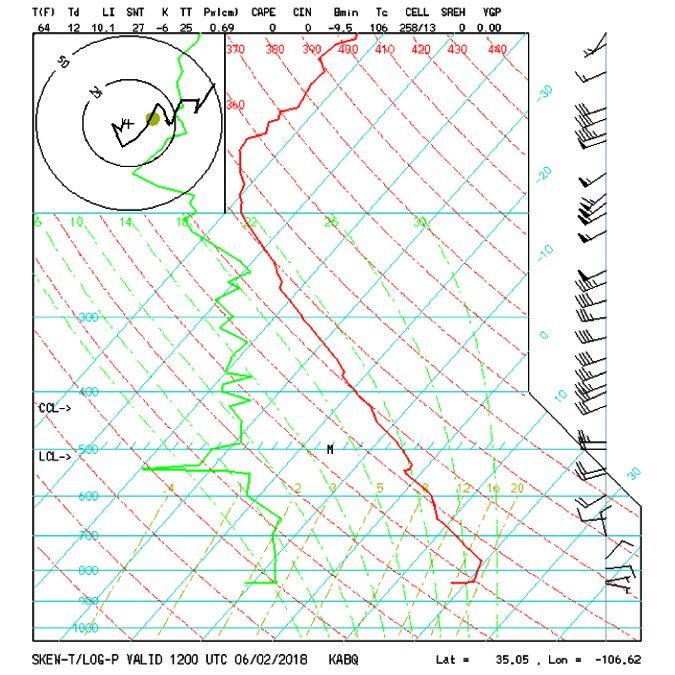
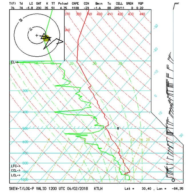
Let me share with you how I, as a pilot, interpret actual Skew T Log P diagrams and relate them to the TAF’s and METARs.
Various diagrams are shown on the previous two pages with my interpretations. It takes practice to interpret these useful diagrams, but as you get familiar with them they’ll tell you a lot and allow you to infer far more than is apparent from the official weather.
Luca F Bencini-Tibo, while secretly dabbling in thermodynamics, vehemently denies being a TV meteorologist.