
Since I began this column over 10 years ago, I’ve strived to write as though you’re with me in the weather operations center, looking over my shoulder and seeing things from my perspective. Since my entire life after high school has revolved around meteorology, it’s always seemed to me that there’s no better way to help pilots come away with valuable insight and techniques than to take you behind the scenes. This should help you make accurate, informed decisions when the weather closes in around you.
During most of my Air Force career I worked as an aviation forecaster. For many years this was a constant succession of four days on, three days off, with rotating shifts. After driving to work, which was usually in a base operations building co-located with dispatch, we would begin a shift-change briefing. If this was in the morning, the entire weather station would participate, including the observers, the section chief, and the commander. If it was evening, the events would be much more relaxed, with just me and the outgoing forecaster reviewing things.
The outgoing forecaster began by covering the current weather picture. We would go over their forecast, itemize any warnings and advisories and review their expiration times, then discuss special aircraft operations, the morning route packages, and other problems. Once I got settled at the desk, I reviewed the charts, working up my own mental picture of the atmosphere and putting together a forecast. This built up groundwork for a TAF and our flight weather products. This is what we will cover here, and hopefully it will help you as a pilot.
The Upper-Air Charts
You might have heard about the “forecast funnel” that describes how the initial workup is done. Rather than going haphazardly through random charts, the forecast funnel begins with large scale processes and works down to the bits and pieces. This is much the same manner in which a car mechanic would start by looking over the engine and running the car to look for obvious problems, rather than opening the hood and taking things apart.
The top of the forecast funnel is where we start, and it stresses the use of large-scale processes. By large-scale, we refer not only to spatial dimensions but also that of time. In other words we’re looking for patterns on the chart that are large, persistent, and slow moving. These form the framework for the rest of the picture.
The best place to start is with the upper tropospheric charts. Here we use actual charts from the National Weather Service’s AWIPS (Advanced Weather Interactive Processing System). This is the core computer system that has been used by all National Weather Service offices for the past 20 years. So you’re getting a rare look at the sophisticated tools that federal weather forecasters use. This is the real deal. So let’s dig in.
The best upper tropospheric chart to start with is the 300 millibar chart shown on this page. This shows conditions at an altitude where the barometric pressure corresponds to 300 millibars, or 8.86 in Hg. This is usually near 30,000 feet MSL, and is designed to help put us at the jet stream level in our forecast area without going into the stratosphere itself. During the transition seasons and summertime we will select higher levels instead (250 and 200 millibars) since the troposphere grows in depth during the warm season.
Looking over the chart, we see a bunch of black lines. These are isoheights, or geopotential contours. Since the actual height of the 300 millibar surface is heavily influenced by the density of the column of air below, this gives us a rough temperature map of where the atmosphere, in general, is quite cold (low heights) and quite warm (high heights). Not surprisingly, we see a vast area of low height in the polar regions. This is the hemispheric polar vortex: not the big bad polar vortex from television weather, but a permanent, extensive feature centered on both poles. On this chart, the polar vortex takes up almost the entire chart, because it drives the prevailing westerlies in the United States.
On the other hand, the tropics are made up of a massive, semi-permanent subtropical ridge that forms a belt around the earth roughly between 30 degrees north and 30 degrees south. If you want to see it, just look at the entire left edge and bottom edge of the chart: these areas are deep within the subtropical ridge.
Closer to the United States we look for lobes of the subtropical ridge that are of immediate interest. The most significant one is at , covering the Gulf of Mexico and the Caribbean. The large expanse of the subtropical ridge is strongly correlated with warm VFR weather. Thunderstorms, showers, and other deep convection are rare. During the summertime, lobes of the subtropical ridge often build into the United States and are commonly associated with heat waves.
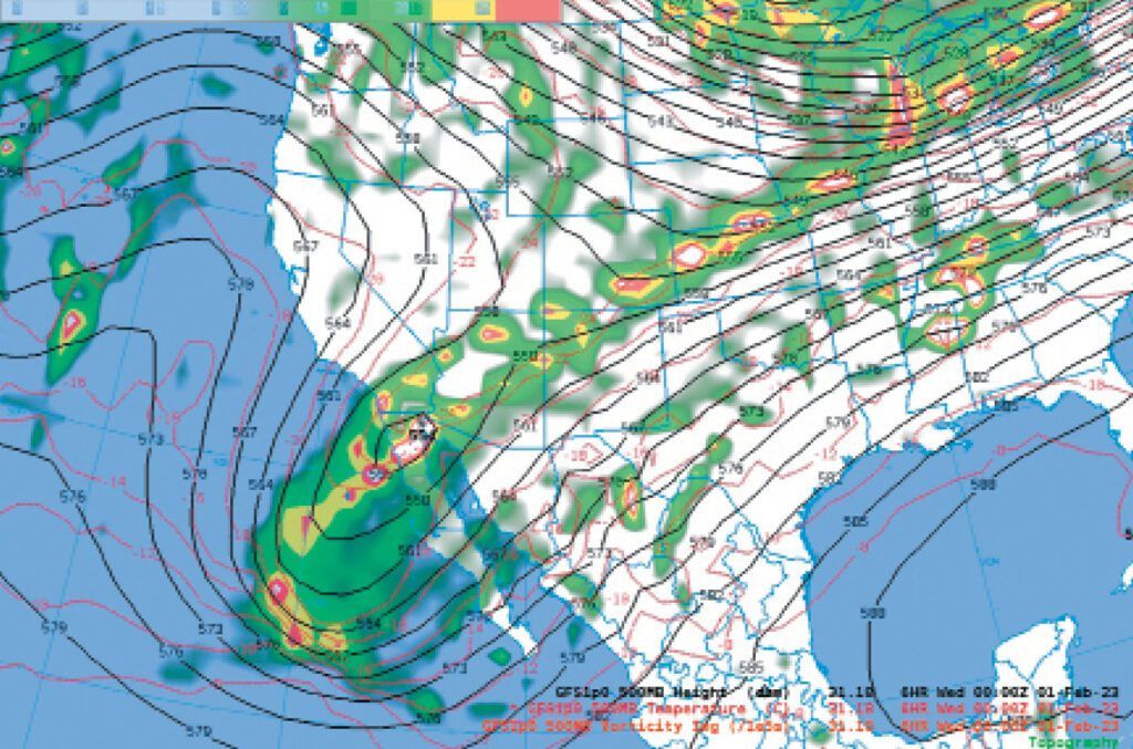
In a similar manner we look for lobes of the polar vortex and areas where it breaks up into smaller circulations. A very prominent example is the large polar low over the Hudson Bay . While it only measures 2000 miles across, it is a smaller, more intense circulation and is closer to what the news media describes as the “polar vortex.” While you might be thinking that this feature is a strong storm system, it’s more correct to describe it as a large area of extremely cold troposphere. This has the potential for frozen fuel in some aircraft.
Another polar low is found in the Gulf of Alaska . We can see that it’s not very deep at all and almost opens up into a trough. This is actually part of an occlusion, and is closer to the jet stream and more likely to be associated with bad weather.
Speaking of the jet stream, let’s look at the gradient, or the packing of the contours. Lines packed close together indicate a strong height (or pressure) differential, implying a strong pressure gradient. If your ground school instructor covered all the important stuff, you’ll know that this means strong winds. And it’s here that we find the jet stream.
You might be thinking that if a cold troposphere and warm troposphere are close together, that puts the upper level highs and lows close together, and pushes the contours closer, making the winds stronger. That’s correct. And it’s what provides the potential energy to power the jet stream winds.
The jet stream is indicated by colored shading, with green indicating winds of 100 knots, yellow of 120 knots, red for 140 knots, and white for 160 knots. The strongest winds in our example are over Ohio and Pennsylvania , with jet stream winds of 160 knots. Indeed a quick check of flight trackers showed that the JFK to LAX flights were angling north over Lake Huron to avoid the winds, while some flights chose to plow directly into the wind, averaging 320-knot groundspeeds and extended block times.
These winds represent the polar front jet. The strongest winds are called the “jet max” or “jet streak” and are usually found directly west of deep surface lows. In fact the area to the east, where the jet max opens up, is referred to as the “exit region” and is closely tied to the location of strong surface systems and bad weather. In this example, this area is off the coast of Maine and near Nova Scotia.
Finally working our way down the forecast funnel, we see smaller waves known as short waves and medium waves. Troughs are found where the contours point southward and contain low values of geopotential height. The region along and east of troughs is associated with bad weather. The most important example is at . This is a deep trough that is moving west to east toward Texas with the prevailing flow. Weather hazards can be expected in the south-central states during the next 48 hours.
Also we find short-wave and medium-wave ridges, which point northward and contain high geopotential height. The best example is at approaching the Pacific Northwest. Good weather is frequently along and ahead of these smaller-scale ridges, so when you see these approaching, chances are you’ll have a relaxing day flying the local pattern.
There are even smaller-scale troughs that are important and contain more intense circulations. They measure from tens to a few hundred miles in size. These are the true short waves, and they do not show up on the 300 millibar chart. Forecasters have to turn to the 500 millibar chart (about 18,000 feet MSL) where they show up better. Diagnostic tools like vorticity, Q vectors, and three-hour pressure falls are essential for helping reveal these features as seen in the chart on the previous page. While these tools are too complex to discuss here and are not always reliable, you can often uncover short waves on your own by locating bands of organized precipitation on radar and well-defined, compact cloud fields approaching your area.
The Surface Chart
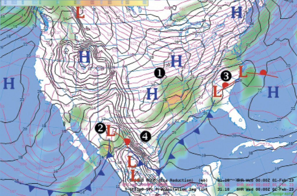
The forecaster then turns his or her attention to the surface chart, above. Again this chart is similar to what you would see at a National Weather Service forecast desk. Isobars (lines of equal pressure) are in black. The red lines indicate 1000-500 millibar thickness. This is a direct measure of atmospheric density in a layer between roughly the surface and 18,000 feet MSL, so in a sense it measures the average temperature in that particular layer. Because of this, we use these red lines for delineating the shape and extent of individual air masses.
The pressure field is dominated by a large surface high . This represents bitterly cold air moving out of Canada. Many other large highs are found on the map. There’s a stagnant plateau high over the Great Basin region, an oceanic high off the coast of California, and an older high over the Bermuda Triangle that represents modified polar air transitioning into warmer air over the Gulf Stream waters. Obviously there’s a lot taking place.
An unusual feature for the Southwest region is the deep low crossing the Rockies in northwest Mexico . This low is a Pacific low that is crossing over to the eastern states, but at a very low latitude. Why so far south? We only need to look at the red lines, and it becomes apparent there’s a large volume of cold air across the United States that’s displacing the storm track well to the south.
The low pressure area is part of the polar front that extends across Mexico into the Gulf. Further to the east it joins up with another wave . This is an older frontal low that migrated across Texas and the Southeast states sometime earlier, where it produced wintry weather from Dallas up to Nashville. When lows reach this part of the country, they have to be watched rather carefully during the wintertime for the development of a coastal low or nor’easter. This becomes less of a concern during the warm season since the air mass temperature contrasts are much weaker.
The weather map shows extensive ridging pointed southward from the high over Oklahoma. If you’re familiar with the terrain in Texas and Mexico, you can sort of visualize this ridge being banked up against the mountains of old Mexico and New Mexico. This is literally “cold air damming,” where shallow cold air has pushed westward against the mountains without crossing over. It has also pushed south into northeast Mexico.
This damming of the cold air is entrenched over these areas, and not even a deep surface low can easily dislodge it. Because of this, forecasters will watch for such a surface low in Mexico to eventually lose definition and “ride over” the top of the cold air as it moves east. Then, it will enter the Gulf of Mexico and redevelop if the upper dynamics cause it to link up with the polar front.
While the weather system crosses the ridge, weather in Texas and the Gulf coast will go downhill and low ceilings and precipitation will develop. Meanwhile forecasters in Florida will be alert to the possibility of a surface low approaching from the west. If the low deepens rapidly in the Gulf, a squall line can develop and move across Florida. One of the strongest such events took place in March 1993, producing a nighttime tornado outbreak across Florida.
Is the TAF Enough?
We’re out of space and have really just scratched the surface of this analysis. These types of charts form the foundation of forecasting, and everything else builds from these basic charts. While you might not need to be a meteorologist to fly safely in unpleasant weather, and you can probably get by with just the TAFs and a thorough briefing, Wx Smarts is here to make you wiser in the ways of aviation meteorology, and now you have a few extra skills in your pocket.
Tim Vasquez was an Air Force aviation forecaster and a forecast systems programmer at Air Force Global Weather Central. His YouTube channel goes into much more depth on these types of charts than possible in this article.


